Advanced Tutorial: Full Pipeline using the Lupus Dataset#
This tutorial walks through the complete huCIRA analysis pipeline using the Lupus dataset as an example. It starts from raw, unprocessed data with ENSG symbols and covers data preparation, enrichment analysis, robustness filtering, and visualization. This comprehensive tutorial covers detailed explanations of all parameters, filtering mechanisms, and plotting options.
For minimal working examples, see the quick_start_cytokine_enrichment.ipynb, quick_start_CIP_enrichment.ipynb, and quick_start_cell-cell_communication.ipynb tutorials.
# Import core packages and the hucira package.

import os
import time
import warnings

import matplotlib.pyplot as plt
import numpy as np
import pandas as pd
import scanpy as sc
from tqdm import TqdmWarning

import hucira as hc

warnings.simplefilter("ignore", TqdmWarning)

start = time.time()
current_wd = os.getcwd()
print(f"Your current working directory: {current_wd}.")
Your current working directory: /ictstr01/home/icb/jenni.liu/all_projects/cytokine_dict_project/huCIRA/docs/notebooks.
1. Load input data#
The two main input files for the huCIRA analysis are:
the Human Cytokine Dictionary
your query transcriptome dataset. Here, we will download the Lupus dataset. It contains ENSG symbols for transcripts, which need to be converted to HGNC symbols. Additionally, the active layer in the dataset is currently scaled, so the raw counts have to be log-normalized for usage of huCIRA. For convenience, the Lupus data is subsampled to 10%.
The files are saved to or loaded from the current working directory. The path is explicitly specified here, although it’s also the default saving location if left unspecified. Choose your own path (directory to project folder) as the workspace for this analysis.
#### Load the human cytokine dictionary (full version) and the Lupus example adata.

df_hcd_all = hc.load_human_cytokine_dict(save_dir=current_wd, mini_version=False, force_download=False)
adata = hc.load_lupus_data(save_dir=current_wd, force_download=False)
sc.pp.subsample(adata, fraction=0.1, copy=False)
adata
AnnData object with n_obs × n_vars = 126367 × 30172
    obs: 'library_uuid', 'assay_ontology_term_id', 'mapped_reference_annotation', 'is_primary_data', 'cell_type_ontology_term_id', 'author_cell_type', 'cell_state', 'sample_uuid', 'tissue_ontology_term_id', 'development_stage_ontology_term_id', 'disease_state', 'suspension_enriched_cell_types', 'suspension_uuid', 'suspension_type', 'donor_id', 'self_reported_ethnicity_ontology_term_id', 'disease_ontology_term_id', 'sex_ontology_term_id', 'Processing_Cohort', 'ct_cov', 'ind_cov', 'tissue_type', 'cell_type', 'assay', 'disease', 'sex', 'tissue', 'self_reported_ethnicity', 'development_stage', 'observation_joinid'
    var: 'feature_is_filtered', 'feature_name', 'feature_reference', 'feature_biotype', 'feature_length', 'feature_type'
    uns: 'citation', 'default_embedding', 'organism', 'organism_ontology_term_id', 'schema_reference', 'schema_version', 'title'
    obsm: 'X_pca', 'X_umap'
#### Optional for easy workflow:
# Enter celltype column name and condition column name of your query adata, which you can read from previous cell output

your_celltype_colname = "cell_type"
your_contrast_colname = "disease_state"
The Enrichment analysis needs two main pieces of information from the query adata: cell types and experimental (disease) conditions.
Annotations have to be examined manually, because naming convention between objects differ. Compare the cell type annotation of the dictionary with the naming convention of your query adata and re-annotate your query adata’s annotation if necessary.
print(f"All cytokines in dictionary:\n  {df_hcd_all.cytokine.unique()}\n")
print(f"All celltypes in dictionary:\n  {df_hcd_all.celltype.unique()}\n")

print(f"All celltypes in query data:\n  {sorted(adata.obs[your_celltype_colname].unique())}\n")
print(
    f"All experimental states (contrasts/conditions) in query data:\n  {sorted(adata.obs[your_contrast_colname].unique())}\n"
)
All cytokines in dictionary:
  ['4-1BBL' 'ADSF' 'APRIL' 'BAFF' 'C5a' 'CD27L' 'CD30L' 'CD40L' 'CT-1'
 'Decorin' 'EGF' 'EPO' 'FGF-beta' 'FLT3L' 'FasL' 'G-CSF' 'GDNF' 'GITRL'
 'GM-CSF' 'HGF' 'IFN-alpha1' 'IFN-beta' 'IFN-epsilon' 'IFN-gamma'
 'IFN-lambda1' 'IFN-lambda2' 'IFN-lambda3' 'IFN-omega' 'IGF-1'
 'IL-1-alpha' 'IL-1-beta' 'IL-10' 'IL-11' 'IL-12' 'IL-13' 'IL-15' 'IL-16'
 'IL-17A' 'IL-17B' 'IL-17C' 'IL-17D' 'IL-17E' 'IL-17F' 'IL-19' 'IL-1Ra'
 'IL-2' 'IL-20' 'IL-21' 'IL-22' 'IL-23' 'IL-24' 'IL-26' 'IL-27' 'IL-3'
 'IL-31' 'IL-32-beta' 'IL-33' 'IL-34' 'IL-35' 'IL-36-alpha' 'IL-36Ra'
 'IL-4' 'IL-5' 'IL-6' 'IL-7' 'IL-8' 'IL-9' 'LIF' 'LIGHT' 'LT-alpha1-beta2'
 'LT-alpha2-beta1' 'Leptin' 'M-CSF' 'Noggin' 'OSM' 'OX40L' 'PRL' 'PSPN'
 'RANKL' 'SCF' 'TL1A' 'TNF-alpha' 'TPO' 'TRAIL' 'TSLP' 'TWEAK' 'VEGF']

All celltypes in dictionary:
  ['Intermediate_B_cell' 'NKT' 'CD8_Memory_T_cell' 'NK_CD56low' 'CD16_Mono'
 'NK_CD56hi' 'CD8_Naive_T_cell' 'pDC' 'ILC' 'MAIT' 'Naive_B_cell'
 'CD4_Naive_T_cell' 'Treg' 'Plasmablast' 'Granulocyte' 'B_cell'
 'CD4_T_cell' 'HSPC' 'CD8_T_cell' 'CD14_Mono' 'cDC' 'CD4_Memory_T_cell'
 'NK' 'Mono']

All celltypes in query data:
  ['B cell', 'CD4-positive, alpha-beta T cell', 'CD8-positive, alpha-beta T cell', 'classical monocyte', 'conventional dendritic cell', 'lymphocyte', 'natural killer cell', 'non-classical monocyte', 'plasmablast', 'plasmacytoid dendritic cell', 'progenitor cell']

All experimental states (contrasts/conditions) in query data:
  ['flare', 'managed', 'na', 'treated']
To create celltype_combos, enter ordered lists that match the same cell types across different naming conventions in your data vs the human cytokine dictionary. “create_celltype_combos()” can help you to create the right format, but you can also format manually.
# Define celltype_combos, an input parameter for enrichment testing
adata_celltypes = [
    "B cell",
    "CD8-positive, alpha-beta T cell",
    "classical monocyte",
    "non-classical monocyte",
    "natural killer cell",
]

hcd_celltypes = ["B_cell", "CD8_T_cell", "CD14_Mono", "CD16_Mono", "NK_CD56hi"]

celltype_combos = hc.create_celltype_combos(adata_celltypes, hcd_celltypes)
print(celltype_combos)

# Define condition of interest
contrast = ("flare", "treated")
contrast_list = [("flare", "treated"), ("flare", "managed"), ("flare", "na")]
print(contrast)
print(contrast_list)
[('B cell', 'B_cell'), ('CD8-positive, alpha-beta T cell', 'CD8_T_cell'), ('classical monocyte', 'CD14_Mono'), ('non-classical monocyte', 'CD16_Mono'), ('natural killer cell', 'NK_CD56hi')]
('flare', 'treated')
[('flare', 'treated'), ('flare', 'managed'), ('flare', 'na')]
2. Process query data#
The enrichment analysis requires log-normalized expression data, and gene identifiers must be provided as HGNC gene symbols, since the Human Cytokine Dictionary uses HGNC nomenclature.
To prepare your data in the appropriate format:
Preprocess the expression data and apply log normalization.
Convert gene identifiers from Ensembl IDs (ENSG) to HGNC gene symbols.
You may use any preferred method for this conversion; below we provide an example using themygenemodule. Install it in your environment if it’s missing.
# You can see that the active layer is currently storing scaled gene expression.
example_row = adata.X[:5].toarray()
example_row
array([[ 0.        ,  0.        ,  0.        , ...,  0.        ,
        -0.25323954,  0.        ],
       [ 0.        ,  0.        ,  0.        , ...,  0.        ,
        -0.35095528,  0.        ],
       [ 0.        ,  0.        ,  0.        , ...,  0.        ,
        -0.36150452,  0.        ],
       [ 0.        ,  0.        ,  0.        , ...,  0.        ,
        -0.37223315,  0.        ],
       [ 0.        ,  0.        ,  0.        , ...,  0.        ,
        -0.2582687 ,  0.        ]], shape=(5, 30172), dtype=float32)
# Save layers
adata.layers["counts"] = adata.raw.X.copy()
adata.layers["scaled_original_counts"] = adata.X.copy()
adata.X = adata.layers["counts"]

# Basic quality checks:
sc.pp.filter_cells(adata, min_genes=200)
sc.pp.filter_genes(adata, min_cells=3)

# Log-normalize:
sc.pp.normalize_total(adata)
sc.pp.log1p(adata)

adata
AnnData object with n_obs × n_vars = 126343 × 20426
    obs: 'library_uuid', 'assay_ontology_term_id', 'mapped_reference_annotation', 'is_primary_data', 'cell_type_ontology_term_id', 'author_cell_type', 'cell_state', 'sample_uuid', 'tissue_ontology_term_id', 'development_stage_ontology_term_id', 'disease_state', 'suspension_enriched_cell_types', 'suspension_uuid', 'suspension_type', 'donor_id', 'self_reported_ethnicity_ontology_term_id', 'disease_ontology_term_id', 'sex_ontology_term_id', 'Processing_Cohort', 'ct_cov', 'ind_cov', 'tissue_type', 'cell_type', 'assay', 'disease', 'sex', 'tissue', 'self_reported_ethnicity', 'development_stage', 'observation_joinid', 'n_genes'
    var: 'feature_is_filtered', 'feature_name', 'feature_reference', 'feature_biotype', 'feature_length', 'feature_type', 'n_cells'
    uns: 'citation', 'default_embedding', 'organism', 'organism_ontology_term_id', 'schema_reference', 'schema_version', 'title', 'log1p'
    obsm: 'X_pca', 'X_umap'
    layers: 'counts', 'scaled_original_counts'
import mygene

mg = mygene.MyGeneInfo()
results = mg.querymany(adata.var_names.tolist(), scopes="ensembl.gene", fields="symbol", species="human")
df = pd.DataFrame(results)

# Create mapping dict (fallback to Ensembl ID when symbol missing)
ensembl_to_symbol = df.set_index("query")["symbol"].fillna(df["query"]).to_dict()
adata.var["gene_symbol"] = adata.var_names.map(ensembl_to_symbol)
adata.var_names_make_unique()

keep_idx = ~adata.var["gene_symbol"].isna()
adata = adata[:, keep_idx].copy()
dup_idx = adata.var["gene_symbol"].duplicated(keep="first")
adata = adata[:, ~dup_idx].copy()
adata.var_names = adata.var["gene_symbol"]
querying 1-1000...done.
querying 1001-2000...done.
querying 2001-3000...done.
querying 3001-4000...done.
querying 4001-5000...done.
querying 5001-6000...done.
querying 6001-7000...done.
querying 7001-8000...done.
querying 8001-9000...done.
querying 9001-10000...done.
querying 10001-11000...done.
querying 11001-12000...done.
querying 12001-13000...done.
querying 13001-14000...done.
querying 14001-15000...done.
querying 15001-16000...done.
querying 16001-17000...done.
querying 17001-18000...done.
querying 18001-19000...done.
querying 19001-20000...done.
querying 20001-20426...done.
Finished.
7 input query terms found dup hits:
	[('ENSG00000261600', 2), ('ENSG00000234162', 2), ('ENSG00000227110', 2), ('ENSG00000233656', 2), ('E
4 input query terms found no hit:
	['ENSG00000250410', 'ENSG00000168078', 'ENSG00000189144', 'ENSG00000267058']
Pass "returnall=True" to return complete lists of duplicate or missing query terms.
# Check your transcript names. Now, they are in HGNC format and you can start the huCIRA analysis.
adata.var.head()
| feature_is_filtered | feature_name | feature_reference | feature_biotype | feature_length | feature_type | n_cells | gene_symbol | |
|---|---|---|---|---|---|---|---|---|
| gene_symbol | ||||||||
| RPL23AP21 | True | ENSG00000228463 | NCBITaxon:9606 | gene | 457 | transcribed_processed_pseudogene | 2063 | RPL23AP21 |
| LINC01409 | True | LINC01409 | NCBITaxon:9606 | gene | 1089 | lncRNA | 570 | LINC01409 |
| FAM87B | True | FAM87B | NCBITaxon:9606 | gene | 1960 | lncRNA | 20 | FAM87B |
| LINC00115 | True | LINC00115 | NCBITaxon:9606 | gene | 874 | lncRNA | 844 | LINC00115 |
| FAM41C | True | FAM41C | NCBITaxon:9606 | gene | 919 | lncRNA | 1193 | FAM41C |
3. Run enrichment analysis#
run_all_enrichment_test() is a wrapper around the core function run_one_enrichment_test(). It runs enrichment analyses across multiple cell types and over a range of filtering parameters, allowing you to assess how robust your results are. If you only need to analyze a single cell type with fixed parameters, you can use run_one_enrichment_test() directly.
Gene set construction#
Before running GSEA, gene sets (signatures) are built from the cytokine dictionary by filtering for differentially expressed genes. Three thresholds control which genes make it into a gene set. Higher values for these parameters produce smaller, more specific gene sets, potentially more precise but at the risk of dropping below min_size.
threshold_lfc— minimum log-fold change a gene must show in response to a cytokine.threshold_expression— minimum expression level, filtering out lowly expressed genes.threshold_pval— maximum adjusted p-value, keeping only statistically significant genes.
With run_all_enrichment_test(), you can pass lists of values for threshold_lfc and threshold_expression to sweep over multiple filtering stringencies at once. This helps you gauge how sensitive your results are to the choice of these thresholds. This will later be important when computing robustness of results: Passing multiple values like threshold_lfc=[0.5, 0.8, 1.0, 1.5] generates multiple gene sets per cytokine. The robustness functions then assess whether enrichment is consistent across these variations. You can choose to run enrichment analyses either for upregulated or downregulated signals.
GSEA parameters#
The enrichment analysis is based on pre-rank Gene Set Enrichment Analysis (GSEA). A few parameters control how it runs:
min_size/max_size— gene sets smaller or larger than these bounds are excluded.permutation_num— number of permutations for estimating p-values. More permutations give more stable results but take longer.weight— controls how much the gene-level ranking metric influences the enrichment score. The default of 1.0 is standard weighted GSEA; setting it to 0.0 gives an unweighted statistic.seed— random seed for reproducibility.
Ranking statistic#
By default, genes are ranked using the signal-to-noise ratio (SNR), which measures how large the expression difference between two groups is relative to the variability within each group. If you prefer a different ranking metric, you can pass your own function via ranking_statistic_fn. More details on how to do define your custom metric can be found in the quick start tutorial quick_start_cytokine_enrichment.ipynb.
# Enrichment analysis for one contrast

enrichment_results = hc.run_all_enrichment_test(
    adata=adata,
    df=df_hcd_all,
    contrast_combo=contrast,
    celltype_combos=celltype_combos,
    contrast_column=your_contrast_colname,
    celltype_column=your_celltype_colname,
    # The following parameters are optional (they have default specifications)
    direction="upregulated",
    # Filtering parameters for gene set construction (of dictionary or gene program)
    threshold_lfc=1.0,
    threshold_expression=0.0,
    threshold_pval=0.01,
    # GSEA parameters
    min_size=10,
    max_size=1000,
    permutation_num=1000,
    weight=1.0,
    seed=2025,
    ranking_statistic_fn=None,
)

# Look at all enrichment results (reduced view to columns of interest, not all statistics)
enrichment_results[
    [
        "celltype_combo",
        "cytokine",
        "contrast",
        "direction",
        "ES",
        "NES",
        "NOM p-val",
        "FDR q-val",
        "FWER p-val",
        "frac_shared_genes_signature",
        "Lead_genes",
        "threshold_lfc",
        "threshold_expression",
    ]
].sort_values("NES", ascending=False).head()
| celltype_combo | cytokine | contrast | direction | ES | NES | NOM p-val | FDR q-val | FWER p-val | frac_shared_genes_signature | Lead_genes | threshold_lfc | threshold_expression | |
|---|---|---|---|---|---|---|---|---|---|---|---|---|---|
| 0 | classical monocyte (CD14_Mono) | IL-6 | flare_vs_treated | upregulated | 0.503346 | 1.591792 | 0.005445 | 0.017648 | 0.045 | 0.892857 | ENPP2;VCAN;MS4A4A;KCNJ15;OLFML2B;GPR34;LINC026... | 1.0 | 0.0 |
| 2 | classical monocyte (CD14_Mono) | IL-10 | flare_vs_treated | upregulated | 0.370541 | 1.409779 | 0.003257 | 0.049564 | 0.206 | 0.852174 | CD14;RGS2;TXLNB;PTGFRN;SCARB1;SCD;KCNMB4;SPIRE... | 1.0 | 0.0 |
| 5 | classical monocyte (CD14_Mono) | IL-21 | flare_vs_treated | upregulated | 0.553939 | 1.278504 | 0.167984 | 0.082107 | 0.435 | 0.650000 | FCGR1A;ENPP2;C1orf21;ABLIM3;ABHD17C;FAM20A | 1.0 | 0.0 |
| 5 | non-classical monocyte (CD16_Mono) | IL-10 | flare_vs_treated | upregulated | 0.367412 | 1.238451 | 0.039683 | 0.585217 | 0.62 | 0.871186 | RFLNB;CAMKK1;PVR;S100A9;FPR1;ATP13A3;ZNRF1;INP... | 1.0 | 0.0 |
| 2 | B cell (B_cell) | IL-21 | flare_vs_treated | upregulated | 0.465881 | 1.223775 | 0.170391 | 1.0 | 0.645 | 0.914286 | BATF;FURIN;SLC2A5;LMO2;LINC02156;BUB1;LINC0241... | 1.0 | 0.0 |
You can combine results from multiple experimental conditions into a single DataFrame by looping over all contrasts of interest. The variable contrast_list was defined in Section 1. This can be useful if you want to aggregate or export results, or perform downstream analyses such as plotting multiple heatmaps side by side. For this tutorial, however, most steps focus on evaluating one contrast at a time.
# To run enrichment analysis for several contrasts, loop through all contrast conditions you are interested in.

all_results = []
for contrast in contrast_list:
    enrichment_df = hc.run_all_enrichment_test(
        adata=adata,
        df=df_hcd_all,
        contrast_combo=contrast,
        celltype_combos=celltype_combos,
        contrast_column=your_contrast_colname,
        celltype_column=your_celltype_colname,
        direction="upregulated",
        threshold_lfc=1.0,
        threshold_expression=0.0,
        threshold_pval=0.01,
        min_size=10,
        max_size=1000,
        permutation_num=1000,
        weight=1.0,
        seed=2025,
        ranking_statistic_fn=None,
    )
    all_results.append(enrichment_df)
multi_contrast_enrichment_results = pd.concat(all_results, ignore_index=True)

# Look at all enrichment results (reduced view to columns of interest, not all statistics)
multi_contrast_enrichment_results[
    [
        "celltype_combo",
        "cytokine",
        "contrast",
        "direction",
        "ES",
        "NES",
        "NOM p-val",
        "FDR q-val",
        "FWER p-val",
        "frac_shared_genes_signature",
        "Lead_genes",
        "threshold_lfc",
        "threshold_expression",
    ]
].sort_values("NES", ascending=False)
| celltype_combo | cytokine | contrast | direction | ES | NES | NOM p-val | FDR q-val | FWER p-val | frac_shared_genes_signature | Lead_genes | threshold_lfc | threshold_expression | |
|---|---|---|---|---|---|---|---|---|---|---|---|---|---|
| 232 | natural killer cell (NK_CD56hi) | IFN-beta | flare_vs_na | upregulated | 0.806282 | 2.530997 | 0.0 | 0.0 | 0.0 | 0.877419 | IFI44L;ISG15;IFITM1;LY6E;IFI6;MX1;IFITM3;XAF1;... | 1.0 | 0.0 |
| 164 | B cell (B_cell) | IFN-beta | flare_vs_na | upregulated | 0.805907 | 2.49256 | 0.0 | 0.0 | 0.0 | 0.904110 | IFI44L;IFITM1;ISG15;MX1;LY6E;EIF2AK2;IFI44;IFI... | 1.0 | 0.0 |
| 233 | natural killer cell (NK_CD56hi) | IFN-omega | flare_vs_na | upregulated | 0.80324 | 2.488184 | 0.0 | 0.0 | 0.0 | 0.875000 | IFI44L;ISG15;LY6E;MX1;PRF1;IFITM3;XAF1;IFI44;G... | 1.0 | 0.0 |
| 177 | CD8-positive, alpha-beta T cell (CD8_T_cell) | IFN-gamma | flare_vs_na | upregulated | 0.880601 | 2.468958 | 0.0 | 0.0 | 0.0 | 0.904110 | IFI44L;IFITM1;ISG15;IFI6;MX1;IFI44;EIF2AK2;OAS... | 1.0 | 0.0 |
| 178 | CD8-positive, alpha-beta T cell (CD8_T_cell) | IL-2 | flare_vs_na | upregulated | 0.812445 | 2.450793 | 0.0 | 0.0 | 0.0 | 0.922156 | IFI44L;IFITM1;ISG15;LY6E;IFI6;GZMH;PRF1;GZMB;M... | 1.0 | 0.0 |
| ... | ... | ... | ... | ... | ... | ... | ... | ... | ... | ... | ... | ... | ... |
| 47 | non-classical monocyte (CD16_Mono) | C5a | flare_vs_treated | upregulated | -0.785597 | -1.820491 | 0.002381 | 0.010364 | 0.005056 | 0.818182 | CTSL;ADM;SLC16A10;HS3ST1;LGALS1;LILRA2 | 1.0 | 0.0 |
| 15 | CD8-positive, alpha-beta T cell (CD8_T_cell) | IFN-gamma | flare_vs_treated | upregulated | -0.54836 | -1.908967 | 0.0 | 0.0 | 0.0 | 0.904110 | ISG15;IFI6;IFITM1;ISG20;TYMP;MX1;IFI44L;EPSTI1... | 1.0 | 0.0 |
| 191 | classical monocyte (CD14_Mono) | TL1A | flare_vs_na | upregulated | -0.83048 | -1.965004 | 0.0 | 0.005078 | 0.002103 | 0.611111 | MT-CO2;DUSP1;CSF1 | 1.0 | 0.0 |
| 14 | CD8-positive, alpha-beta T cell (CD8_T_cell) | IFN-alpha1 | flare_vs_treated | upregulated | -0.716089 | -2.157756 | 0.0 | 0.0 | 0.0 | 0.942857 | ISG15;IFI6;TYMP;MX1;IFI44L;EPSTI1;IRF7;IFIT1;L... | 1.0 | 0.0 |
| 13 | CD8-positive, alpha-beta T cell (CD8_T_cell) | IL-1-beta | flare_vs_treated | upregulated | -0.689024 | -2.215796 | 0.0 | 0.0 | 0.0 | 0.937500 | RPL18A;ISG15;MT-CO1;IFI6;MT-CO2;IFITM1;TYMP;PI... | 1.0 | 0.0 |
246 rows × 13 columns
CIP enrichment#
Cytokine-induced gene program enrichment analysis is ran in a very similar way. Please refer to the quick_start_CIP_enrichment.ipynb tutorial for details.
4. Identify robust and significant results#
Since run_all_enrichment_test() runs enrichment across multiple filtering thresholds, each cytokine–cell type pair can produce several results — one per parameter combination. This lets us assess whether a result holds up across different gene set constructions or only appears under one specific setting.
Robustness and significance are determined by two criteria:
Is the result evaluable often enough? Depending on the filtering thresholds, some gene sets may end up too small (or too large) for GSEA to run (see
min_size/max_sizeinrun_all_enrichment_test). Thethreshold_validparameter sets the minimum fraction of parameter combinations that must yield a valid result. Cytokines that are only evaluable under very few settings are discarded.Is the result significant often enough? Among the valid results,
threshold_below_alphasets the minimum fraction that must be significant (based on the FDR q-value). A cytokine that is only significant under one particular filtering setting is less reliable than one that is consistently significant across many.
Results passing both criteria are considered robust. They hold up across different gene set constructions rather than depending on a single parameter choice.
Two functions apply these criteria:
check_robustnessfilters for a single q-value threshold and directly returns the filtered enrichment results.get_robust_significant_resultsadditionally sweeps over three significance thresholds (alphas), which get assigned signficance stars. By default, alphas will represent [0.1, 0.05, 0.01]. Returns three DataFrames, the first two of which are used for plotting the enrichment heatmap. The main difference tocheck_robustnesslies in its generation of functional and plot-ready outputs.
robust_results = hc.check_robustness(
    enrichment_results,
    threshold_qval=0.01,  # direct impact on NES results: filters FDR q-val
    threshold_valid=0.1,
    threshold_below_alpha=0.9,
)
robust_results
| celltype_combo | contrast | cytokine | frac_valid | frac_significant | is_robust | NES_min | NES_max | FDR q-val | qval_threshold | threshold_frac_below_alpha | |
|---|---|---|---|---|---|---|---|---|---|---|---|
| 0 | CD8-positive, alpha-beta T cell (CD8_T_cell) | flare_vs_treated | IL-1-beta | 1.0 | 1.0 | True | -2.215796 | -2.215796 | 0.0 | 0.01 | 0.9 |
| 1 | CD8-positive, alpha-beta T cell (CD8_T_cell) | flare_vs_treated | IFN-alpha1 | 1.0 | 1.0 | True | -2.157756 | -2.157756 | 0.0 | 0.01 | 0.9 |
| 2 | CD8-positive, alpha-beta T cell (CD8_T_cell) | flare_vs_treated | IFN-gamma | 1.0 | 1.0 | True | -1.908967 | -1.908967 | 0.0 | 0.01 | 0.9 |
nes_plot_df, annot_plot_df, robust_results = hc.get_robust_significant_results(
    results=enrichment_results,
    alphas=[0.1, 0.05, 0.01],
    threshold_valid=0.1,
    threshold_below_alpha=0.9,
    display_robust_results=True,
)
| contrast | celltype_combo | cytokine | qval_threshold | |
|---|---|---|---|---|
| 0 | flare_vs_treated | CD8-positive, alpha-beta T cell (CD8_T_cell) | IFN-alpha1 | 0.01 |
| 1 | flare_vs_treated | CD8-positive, alpha-beta T cell (CD8_T_cell) | IFN-beta | 0.05 |
| 2 | flare_vs_treated | CD8-positive, alpha-beta T cell (CD8_T_cell) | IFN-gamma | 0.01 |
| 3 | flare_vs_treated | CD8-positive, alpha-beta T cell (CD8_T_cell) | IFN-omega | 0.05 |
| 4 | flare_vs_treated | CD8-positive, alpha-beta T cell (CD8_T_cell) | IL-1-beta | 0.01 |
| 5 | flare_vs_treated | CD8-positive, alpha-beta T cell (CD8_T_cell) | IL-15 | 0.05 |
| 6 | flare_vs_treated | CD8-positive, alpha-beta T cell (CD8_T_cell) | IL-2 | 0.05 |
| 7 | flare_vs_treated | CD8-positive, alpha-beta T cell (CD8_T_cell) | IL-27 | 0.05 |
| 8 | flare_vs_treated | CD8-positive, alpha-beta T cell (CD8_T_cell) | IL-7 | 0.05 |
| 9 | flare_vs_treated | classical monocyte (CD14_Mono) | IL-10 | 0.05 |
| 10 | flare_vs_treated | classical monocyte (CD14_Mono) | IL-21 | 0.10 |
| 11 | flare_vs_treated | classical monocyte (CD14_Mono) | IL-6 | 0.05 |
| 12 | flare_vs_treated | non-classical monocyte (CD16_Mono) | C5a | 0.05 |
You can see that the output robust_results contains similar information for both functions. However, get_robust_significant_results returns a set of enrichment results that pass at least one of the three qval_thresholds (alphas). All output dataframes from get_robust_significant_results are then used as input for the plotting function. In particular, take a look at nes_plot_df and annot_plot_df, which will be visualized as a heatmap in the next section.
nes_plot_df
| celltype_combo | B cell (B_cell) | CD8-positive, alpha-beta T cell (CD8_T_cell) | classical monocyte (CD14_Mono) | natural killer cell (NK_CD56hi) | non-classical monocyte (CD16_Mono) |
|---|---|---|---|---|---|
| cytokine | |||||
| C5a | NaN | NaN | -0.804926 | NaN | -1.820491 |
| CD40L | -0.747786 | NaN | NaN | NaN | NaN |
| GM-CSF | NaN | NaN | -1.181667 | NaN | 0.986207 |
| IFN-alpha1 | NaN | -2.157756 | -1.408583 | NaN | -1.301530 |
| IFN-beta | -0.949559 | -1.521071 | -1.088863 | -1.324211 | -1.272691 |
| IFN-gamma | 0.838154 | -1.908967 | -0.978505 | -1.176742 | 0.951379 |
| IFN-omega | -0.901971 | -1.489039 | -1.072829 | -1.356344 | -1.177617 |
| IL-1-alpha | NaN | NaN | -1.132500 | NaN | -1.434384 |
| IL-1-beta | -1.524112 | -2.215796 | -0.943179 | -0.881689 | -1.200225 |
| IL-10 | 0.721797 | NaN | 1.409779 | -1.092695 | 1.238451 |
| IL-12 | NaN | NaN | 0.966729 | 1.093809 | -1.113725 |
| IL-13 | 1.047150 | NaN | 0.871762 | NaN | -0.912971 |
| IL-15 | 0.767731 | -1.390675 | -1.194397 | 0.939899 | -0.996253 |
| IL-2 | -0.837790 | -1.448697 | -1.065552 | 1.039084 | -1.247886 |
| IL-21 | 1.223775 | NaN | 1.278504 | 1.062732 | 0.851697 |
| IL-27 | NaN | -1.517245 | NaN | NaN | NaN |
| IL-3 | NaN | NaN | -1.209489 | NaN | 0.851473 |
| IL-32-beta | 0.903246 | 1.042213 | -0.992106 | 1.073143 | -1.016514 |
| IL-4 | 0.954229 | -0.815442 | -0.950532 | 0.841600 | 0.826358 |
| IL-6 | NaN | NaN | 1.591792 | NaN | 0.958220 |
| IL-7 | -1.335636 | -1.422273 | -1.247765 | 1.163014 | -1.055112 |
| Leptin | NaN | NaN | -1.327519 | -1.225018 | NaN |
| M-CSF | NaN | NaN | -1.154549 | NaN | -1.083629 |
| TL1A | NaN | NaN | -1.483487 | NaN | NaN |
| TSLP | NaN | NaN | -1.203972 | 1.120691 | -0.992963 |
annot_plot_df
| celltype_combo | B cell (B_cell) | CD8-positive, alpha-beta T cell (CD8_T_cell) | classical monocyte (CD14_Mono) | natural killer cell (NK_CD56hi) | non-classical monocyte (CD16_Mono) |
|---|---|---|---|---|---|
| cytokine | |||||
| C5a | ** | ||||
| CD40L | |||||
| GM-CSF | |||||
| IFN-alpha1 | *** | ||||
| IFN-beta | ** | ||||
| IFN-gamma | *** | ||||
| IFN-omega | ** | ||||
| IL-1-alpha | |||||
| IL-1-beta | *** | ||||
| IL-10 | ** | ||||
| IL-12 | |||||
| IL-13 | |||||
| IL-15 | ** | ||||
| IL-2 | ** | ||||
| IL-21 | * | ||||
| IL-27 | ** | ||||
| IL-3 | |||||
| IL-32-beta | |||||
| IL-4 | |||||
| IL-6 | ** | ||||
| IL-7 | ** | ||||
| Leptin | |||||
| M-CSF | |||||
| TL1A | |||||
| TSLP |
5. Plotting#
huCIRA provides two plotting functions: plot_significant_results visualizes the enrichment results in heatmaps and plot_communication plots cytokine-mediated cell-cell communication.
Enrichment heatmap#
plot_significant_results() plots a heatmap of the robust enrichment results. Each cell shows the mean NES across parameter combinations, and significance is annotated with stars (*, **, ***) based on the alphas defined in get_robust_significant_results. The heatmap takes the outputs nes_plot_df and annot_plot_df as input. Optionally, robust_results can be provided as well to define the plotted contrast conditions.
You can subset the plot to specific cytokines or cell types using selected_cytokines and selected_celltypes. Use fontsize, fig_width, and fig_height to adjust the appearance. Set save_fig=True to save the figure as an .svg file to the directory specified by fig_path.
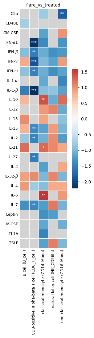
hc.plot_significant_results(
    nes_plot_df=nes_plot_df,
    annot_plot_df=annot_plot_df,
    robust_results=robust_results,
    selected_celltypes=None,
    selected_cytokines=None,
    fontsize=9,
    save_fig=False,
    fig_path="",
    fig_width=10.0,
    fig_height=10.0,
)
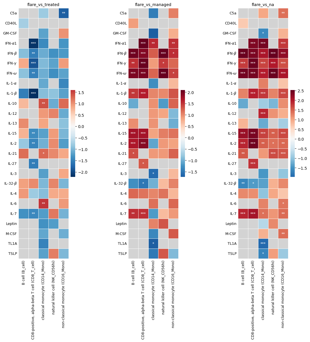
Earlier, we ran enrichment analyses over several contrast conditions, which returned the dataframe multi_contrast_enrichment_results. To visualize enrichment results across contrasts, you can plot multiple heatmaps side by side. You can do this manually by looping through the contrast conditions. Pass an ax argument to plot_significant_results to draw into a specific subplot. Otherwise, they will be plotted separately. If no robust results exist for a contrast, the subplot is left empty.
fig, axes = plt.subplots(1, 3, figsize=(12, 12))

for idx, contrast in enumerate(multi_contrast_enrichment_results.contrast.unique()):
    print(contrast)
    nes_plot_df, annot_plot_df, robust_results = hc.get_robust_significant_results(
        results=multi_contrast_enrichment_results,
        contrast_combo=contrast,
        alphas=[0.1, 0.05, 0.01],
        threshold_valid=0.1,
        threshold_below_alpha=0.9,
        display_robust_results=False,
    )

    if robust_results is not None and not robust_results.empty:
        hc.plot_significant_results(
            nes_plot_df,
            annot_plot_df,
            robust_results,
            ax=axes[idx],
            fontsize=9,
        )
    else:
        axes[idx].set_axis_off()
        axes[idx].set_title(f"{contrast}\nNo robust significant results")

plt.tight_layout()
plt.subplots_adjust(wspace=0.01)
plt.show()
flare_vs_treated
flare_vs_managed
flare_vs_na
Cell-cell communication: compute senders and receivers#
get_all_senders_and_receivers() identifies which cell types produce a cytokine (senders) and which express its receptor (receivers). Pass in the list of cytokines you want to analyze via cytokine_list, typically the robust cytokines from the enrichment analysis, or a custom set. They must be present in the cytokine information file to define sender and receiver relationships. The function will then identify which genes are in your query data as well.
sender_pvalue_threshold— maximum p-value (from a Wilcoxon rank-sum test across cell types) for a cell type to be considered a sender. Only cell types where the cytokine gene is significantly more expressed compared to other cell types are included.receiver_mean_X_threshold— minimum mean receptor gene expression for a cell type to be considered a receiver. Set to 0 to include all cell types with any detectable receptor expression.
cytokine_info = hc.load_cytokine_info()
cytokine_info.head()
| Unnamed: 0 | name | gene | used cytokines | DEG_plot_family | single_family | family_level_1 | family_level_2 | receptor gene | alternative names | comments | parse_cytokine | single_gene | go_annotations | go_labels | functional_classification | |
|---|---|---|---|---|---|---|---|---|---|---|---|---|---|---|---|---|
| 0 | 0 | IL-1-alpha | IL1A | IL-1α | IL-1 | IL-1 | interleukin | IL-1 | IL1R1, IL1RAP | Interleukin 1 alpha | NaN | True | IL1A | ['GO:0005125', 'GO:0046688', 'GO:0034605', 'GO... | cytokine activity, extracellular space, positi... | Pro-inflammatory |
| 1 | 1 | IL-1-beta | IL1B | IL-1β | IL-1 | IL-1 | interleukin | IL-1 | IL1R1, IL1RAP | Interleukin 1 beta | NaN | True | IL1B | ['GO:0005125', 'GO:0070372', 'GO:0001934', 'GO... | cytokine activity, positive regulation of prot... | Pro-inflammatory |
| 2 | 2 | IL-1Ra | IL1RN | IL-1Ra | IL-1 | IL-1 | interleukin | IL-1 | IL1R1 | Interleukin 1 receptor antagonist | NaN | True | IL1RN | ['GO:0006953', 'GO:0005813', 'GO:0005149', 'GO... | extracellular space, protein binding, cytosol,... | Anti-inflammatory |
| 3 | 3 | IL-18 | IL18 | IL-18 | IL-1 | IL-1 | interleukin | IL-1 | IL18R1, IL18RAP | Interleukin 18 | NaN | True | IL18 | ['GO:0005125', 'GO:0005615', 'GO:0032819', 'GO... | cytokine activity, extracellular space, positi... | Pro-inflammatory, Th1-associated |
| 4 | 4 | IL-33 | IL33 | IL-33 | IL-1 | IL-1 | interleukin | IL-1 | IL1RL1, IL1RAP | Interleukin 33 | NaN | True | IL33 | ['GO:0005125', 'GO:0005737', 'GO:0005615', 'GO... | cytokine activity, cytoplasm, extracellular sp... | Pro-inflammatory |
df_senders, df_receivers = hc.get_all_senders_and_receivers(
    adata=adata,
    cytokine_info=cytokine_info,
    cytokine_list=robust_results.cytokine.unique(),
    celltype_colname=your_celltype_colname,
    sender_pvalue_threshold=0.1,
    receiver_mean_X_threshold=0,
)
df_senders.head()
| min_logfoldchanges | min_pvals | min_pvals_adj | gene | mean_X | frac_X | mean_X>0 | cytokine | celltype | |
|---|---|---|---|---|---|---|---|---|---|
| CD8-positive, alpha-beta T cell | 2.76905 | 0.0 | 0.0 | IFNG | 0.054769 | 0.058260 | 0.054769 | IFN-gamma | CD8-positive, alpha-beta T cell |
| lymphocyte | 2.511762 | 0.0 | 0.0 | IFNG | 0.092878 | 0.185006 | 0.092878 | IFN-gamma | lymphocyte |
| natural killer cell | 1.741828 | 0.0 | 0.0 | IFNG | 0.049104 | 0.054678 | 0.049104 | IFN-gamma | natural killer cell |
| classical monocyte | 1.848429 | 0.0 | 0.0 | IL15 | 0.029858 | 0.049086 | 0.029858 | IL-15 | classical monocyte |
| non-classical monocyte | 1.758463 | 0.0 | 0.0 | IL15 | 0.041609 | 0.090384 | 0.041609 | IL-15 | non-classical monocyte |
df_receivers.head()
| mean_X | frac_X | cytokine | celltype | |
|---|---|---|---|---|
| B cell | 0.030110 | 0.045329 | IFN-beta | B cell |
| lymphocyte | 0.054595 | 0.139057 | IFN-beta | lymphocyte |
| natural killer cell | 0.034506 | 0.044113 | IFN-beta | natural killer cell |
| CD4-positive, alpha-beta T cell | 0.042741 | 0.065390 | IFN-beta | CD4-positive, alpha-beta T cell |
| CD8-positive, alpha-beta T cell | 0.037064 | 0.055736 | IFN-beta | CD8-positive, alpha-beta T cell |
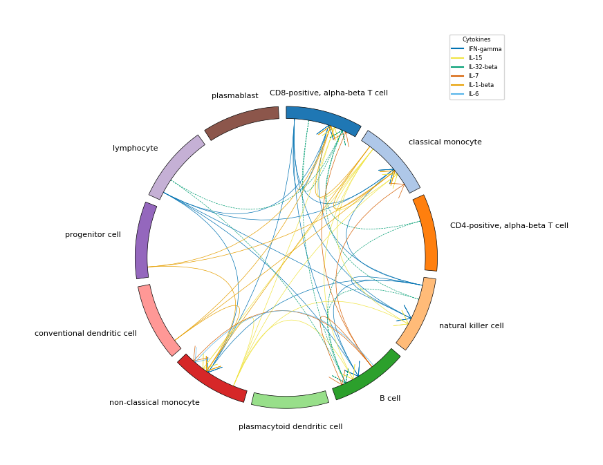
Cell-cell communication circos plot#
plot_communication() visualizes which cell types send and receive cytokine signals using a circos plot. It requires sender and receiver DataFrames computed by get_all_senders_and_receivers(), which identifies for each cytokine which cell types express the cytokine gene (senders) and which express its receptor (receivers). For an overview, refer to quick_start_cell-cell_communication.ipynb.
Filtering communication links#
The circos plot can get crowded when many cell types and cytokines are involved. Several parameters let you filter which communication links are shown:
frac_expressing_cells_sender/frac_expressing_cells_receiver— minimum fraction of cells in a cell type that must express the cytokine gene (sender) or the receptor gene (receiver). This removes links driven by only a handful of cells, which are less likely to reflect real communication.mean_cytokine_gene_expression_sender/mean_cytokine_gene_expression_receiver— minimum mean expression level of the cytokine or receptor gene in a cell type. This filters out cell types where the gene is technically detected but at very low levels. These thresholds should be set in the same scale as your expression data (e.g. log-normalized).df_enrichment— if provided, only cytokines that appear in this DataFrame are plotted. Typically, you pass in the robust enrichment results so that the circos plot only shows cytokines with significant enrichment in at least one cell type.all_celltypes— if not provided, only cell types present in the sender and receiver DataFrames are plotted. In this tutorial, all cell type groups of the query data are passed so that all are visualized.
Appearance#
Colors for cytokines and cell types are assigned automatically, but you can provide your own mappings via cytokine2color and celltype2color. Use figsize to adjust the plot size, lw for the line width of signaling arrows, and fontsize for the labels. loc and bbox_to_anchor control the position of the legend. The figure is only saved if save_path is specified.
# Plots cell-cell communication

expression_threshold = 0.1 / 10_000  # = 100 TPM
expression_threshold = np.log2((expression_threshold) + 1)

legend_handles, legend_labels = hc.plot_communication(
    df_src=df_senders,
    df_tgt=df_receivers,
    df_enrichment=robust_results,
    all_celltypes=np.array(adata.obs[your_celltype_colname].unique()),
    # Filtering statistics
    frac_expressing_cells_sender=0,
    frac_expressing_cells_receiver=0,
    mean_cytokine_gene_expression_sender=expression_threshold,
    mean_cytokine_gene_expression_receiver=expression_threshold,
    # map your custom cytokine and cell type colors as dictionaries
    cytokine2color=None,
    celltype2color=None,
    # Plotting aeshetics
    show_legend=True,
    figsize=(8, 9),
    lw=0.5,
    fontsize=8,
    bbox_to_anchor=(1.1, 1.1),
    loc="center",
    save_path=None,
)
end = time.time()
print(f"Time: {int((end - start) / 60)} min {int((end - start) % 60)} sec")
Time: 6 min 11 sec
## --END-- ##